Basics of Data Manipulation in Python

May 31, 2023 4-minute read

python • numpy • pandas • regex

In this post, we learn the basics of data manipulation in Python. We’ll use the following:

Regular Expressions
Numpy
Pandas

Regular Expression

Let’s start from this string and basic imports:

import re

str = "Hello, World. It's me, Python."

Now we can use regular expressions to get what we’re looking for. For example, we want all words which start from capital letter are of size at least 2:

1
2


pattern = r'[A-Z]\w+'
re.findall(pattern, str)

Output:

['Hello', 'World', 'It', 'Python']

Listing:

1: r'[A-Z]\w+' - r indicates to Python it’s not a normal string. Otherwise, it would treat \ as a special character, like \n - a new line, which wouldn’t be what we want here, as regexp uses them to indicate special meaning, e.g. \w - word character. Next, [A-Z] means that the first letter should be between A - Z, and lastly, + means we want at least one-word character, which together with the first letter give us at least 2 size (asked in the question)

2: Once we have the pattern, we need to apply it to the string. findall gives us a list of all matches.

To learn more about regular expression, we can check the well-written documentation: https://docs.python.org/3/library/re.html

To create complicated regexp, sometimes we want to experiment with them on our test. We can do this, for example here: https://regex101.com/

Even though regexp has a bad press, it may be helpful when we start data preparation.

NumPy

NumPy is a library for scientific computing. It helps in working in large, multi-dimensional arrays and matrices. It also comes with a lot of mathematical functions.

Let’s see it in action:

import numpy as np

print(type([1, 2, 3]))
print(type(np.array([1, 2, 3])))

Output:

<class 'list'>
<class 'numpy.ndarray'>

list is a basic type in Python. It’s very good but has some limitations. Especially in numerical and matrix operations. For example:

[1, 2, 3] + [4, 5, 6]

Output:

[1, 2, 3, 4, 5, 6]

Oh no, interpreting our lists as vectors don’t seem right. Adding two vectors here should be [5, 7, 9].

As we would like to use lots of matrices and vectors and have different mathematical operations, different types must be introduced.

Meet ndarray, which gives you a variety of math functions. Additionally, ndarray is statically typed. The type is known on the creation of the array, whereas with lists, we can keep different types: my_list = [1, 'hello', 3.14]. We say that ndarray is homogeneous.

np.array([1, 2, 3]) + np.array([4, 5, 6])

Output:

[5, 7, 9]

We can do much better:

np.zeros(5) // [0, 0, 0, 0, 0]
np.zeros((2, 3)) // [[0, 0, 0], [0, 0, 0]]
np.random.rand(2, 3) // [[0.1, 0.2, 0.3], [0.4, 0.5, 0.6]] <- random values
np.arange(1, 10, 2) // [1, 3, 5, 7, 9]
np.linspace(0, 1, 5) // [0.0, 0.25, 0.5, 0.75, 1.0]
np.random.rand(4, 2) // random matrix 4x2

and vector operations:

a = np.random.rand(4)
b = np.random.rand(4)

a + b // element-wise addition
a - b // element-wise subtraction
a % 2 // element-wise modulo
a * b // element-wise multiplication
a @ b // dot product

Where dot product is defined as: $$ \mathbf{a} \cdot \mathbf{b} = \sum_{i=1}^{n} a_i b_i $$

Pandas

Series

Pandas, another common library in data science, is built on top of Numpy. It gives us a lot of useful functions for data manipulation.

Series, is one-dimensional ndarray with axis labels:

import pandas as pd

pd.Series(['Alice', 'Bob', 'Molly'])

Output

0    Alice
1     Bob
2    Molly
dtype: object

Initially, I was confused by this type, as it looks exactly like an array. The key here comes with the labels, which may not only be ints but any type, for example, string or datetime.

1
2
3
4
5
6
7
8


s = pd.Series({
    'AAA': 'Alice',
     'BBB': 'Bob',
     'CCC': 'Molly'
})

print(s.iloc[1])
print(s.loc['BBB'])

Output:

Bob
Bob

7-8: iloc integer location index - returns as a row by numeric index, whereas loc label-based index returns a row by a label.

DataFrame

df = pd.DataFrame({
    'A': [1, 2, 3],
    'B': [4, 5, 6],
    'C': [7, 8, 9]
})

Output:

Series was one dimensional labelled array, and DataFrame is a two-dimensional labelled array. It’s like a table in SQL or Excel.

And just like SQL, it provides a lot of useful functions: groupby, join, merge, etc.

Let’s do some practice in DataFrame. For this, I will use Finance Data from Kaggle: https://www.kaggle.com/datasets/nitindatta/finance-data?resource=download

Read the data:

import pandas as pd
import matplotlib.pyplot as plt

df = pd.read_csv('Finance_data.csv') // your path to the csv
print(df.head())

Group and narrow does amount of columns:

df[['gender', 'Mutual_Funds']].groupby('gender').count()

Output:

Female,15
Male,25

Let’s leave only records which have Mutual Funds (and show the first 10 rows):

df[df['Mutual_Funds'] == 1].head(10)

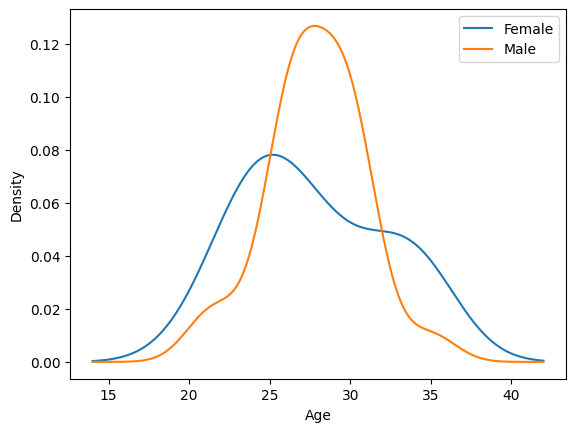
what about drawing a plot, let’s say a gender distribution:

df.groupby('gender').age.plot(kind='kde')
plt.xlabel('Age')
plt.legend()
plt.show()

Output:

Gender distribution