Math Methods in Data Science

In Data Science, understanding some math is essential. Let’s review some essential math methods in Python grouped in:

• Basics
• Linear Algebra
• Probability
• Statistics

Basics

Basic operations on sets

set(range(1, 10)) // a set
mod2 = {x for x in range(1, 10) if x % 2 == 0} // another set
mod3 = {x for x in range(1, 10) if x % 3 == 0} // yet another set

mod2 | mod3 // union
mod2 & mod3 // intersection
mod2 - mod3 // difference

Solving Functions in python are done with sympy

import sympy as sp

x = sp.symbols('x')
y = 2*x + 3

y.diff(x) // first derivative of y with respect to x (dy/dx)

sp.solve(y, x) // solve y = 0 for x

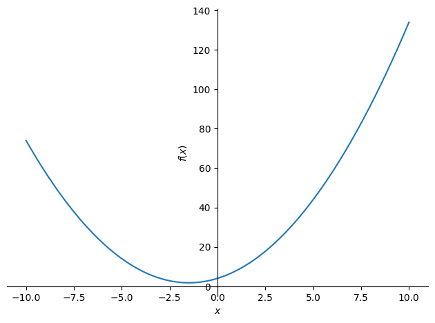
Let’s take more complicated functions and plot it

y = x**2 + 3*x + 4
sp.plot(y)

df_dx = y.diff(x)
df_dx

Output: 2x+3

Now, we can calculate the value in a x=2 point of the derivative:

df_dx.evalf(subs={x: 2})

or find zeros of the derivative:

sp.solve(df_dx, x)

Output: [-3/2]

Linear Algebra

Numpy provies a lot of methods for linear algebra. They are defined in np.linalg module.

Let’s define some vectors:

import numpy as np

v = np.array([10, 20, 30, 40, 50]) // vector 1
w = np.array([1, 2, 3, 4, 5]) // vector 2

There are a few important concepts with vectors and matrices. Firstly, let’s understand the definition and then see how we can calculate it in Python.

• linear combination - a linear combination of vectors v1, v2, …, vn is any vector of the form a1v1 + a2v2 + … + anvn, where a1, a2, …, an are scalars
• span - the span of a set of vectors is the set of all their linear combinations
• basis - a basis of a vector space is a set of vectors that are linearly independent and that span the vector space
• linear independence - a set of vectors is linearly independent if no vector in the set is a linear combination of the other vectors in the set
• rank of a matrix - the maximum number of linearly independent column vectors in the matrix
• dot product - the dot product of two vectors is the sum of the products of the corresponding entries of the two sequences of numbers

np.linalg.matrix_rank(v) // rank of a matrix
v.dot(w) // dot product
v + w
v - w
v * w // element-wise multiplication

and operations on some matrices

matrix = np.random.randn(3, 4)
matrix.shape

Output: (3, 4)

Check linear independence:

rank = np.linalg.matrix_rank(matrix)
is_linear_independence = rank == matrix.shape[0]
is_linear_independence

Output: True

Matrix operations:

A = np.random.randn(3, 4)
B = np.random.randn(4, 5)

A.dot(B) // matrix multiplication
A @ B // or matrix multiplication

np.linalg.det(C) // matrix determinant
np.linalg.inv(C) // matrix inverse

Lastly, we see how we can find eigenvalues and eigenvectors.

A scalar λ is called an eigenvalue of a matrix A if there is a non-zero vector x such that Ax = λx. Such a vector x is called an eigenvector corresponding to λ.

eigvalues, eigvectors = np.linalg.eig(C) // eigenvalues and eigenvectors

Probability

To play with probability we need to import scipy.stats module, and few more:

from scipy.stats import norm
from scipy.stats import rv_discrete
import numpy as np
import matplotlib.pyplot as plt

We can define a very simple random variable:

X = np.random.randint(0, 100) // define random variable between [0, 100)

Let’s define few concepts:

probability mass function - a function that gives the probability that a discrete random variable is exactly equal to some value

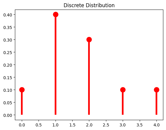
Discrete distribution:

x = np.arange(5)
P_x = [0.1, 0.4, 0.3, 0.1, 0.1]
X = rv_discrete(name='X', values=(x, P_x))

X.pmf(x) // probability mass function

Output: array([0.1, 0.4, 0.3, 0.1, 0.1])

Let’s plot it:

fig, ax = plt.subplots(1, 1)
ax.plot(x, y, 'ro', ms=12, mec='r')
ax.vlines(x, 0, y, colors='r', lw=4)
ax.set_title('Discrete Distribution')

Output:

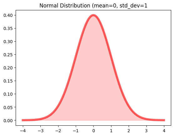
Similarly, for continous distribution:

probability dense function - a function that gives the probability that a continuous random variable would have exactly the value x

mean = 0
std_dev = 1
X = norm(loc=mean, scale=std_dev) // define normal distribution (mean=0, std_dev=1)

x = np.linspace(-4*std_dev, 4*std_dev, 1000)
y = X.pdf(x)

And plot it:

fig, ax = plt.subplots(1, 1)
ax.plot(x, y, 'r-', lw=5, alpha=0.6, label='norm pdf')
ax.fill_between(x, 0, y, alpha=0.2, color='r')
ax.set_title('Normal Distribution (mean=0, std_dev=1')

Output:

To calculate expected values, variance, conditional probability and Bayes’ rule:

X.expect() // expected value
X.var() // variance

A = np.random.choice([True, False], size=10)
B = np.random.choice([True, False], size=10)
p_a_and_b = np.mean(A & B)
p_b = np.mean(B)
p_a_given_b = p_a_and_b / p_b
p_a_given_b

Output: 0.7499999999999999

Bayes’ rule - a way to calculate conditional probability. It is named after Thomas Bayes, who first showed how it worked.

def bayes_rule(p_b_given_a, p_a, p_b):
    return p_b_given_a * p_a / p_b
    
p_b_given_a = 0.5
p_a = 0.1
p_b = 0.4

bayes_rule(p_b_given_a, p_a, p_b)

Output: 0.125

Statistics

Central Limit Theorem

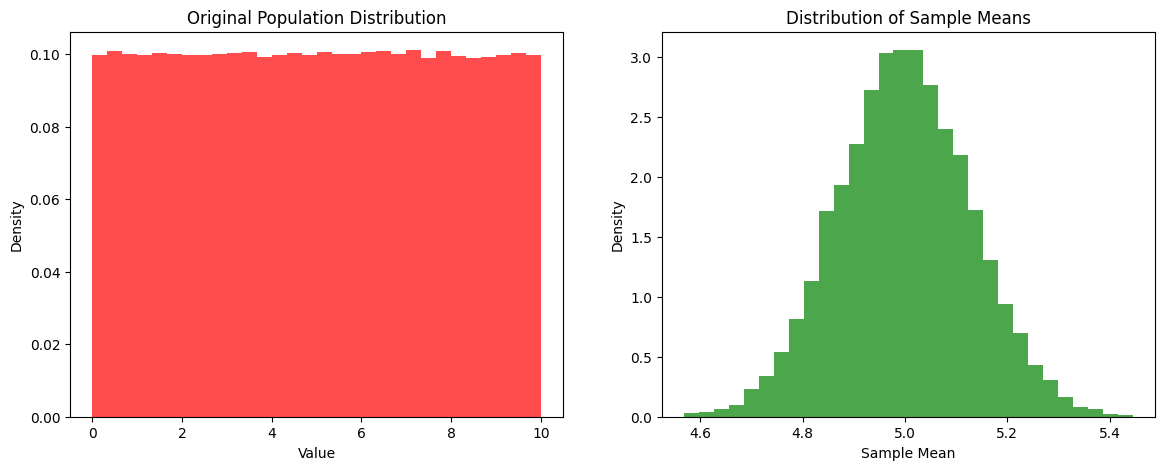
Central Limit Theorem - the sum of a large number of independent random variables will be approximately normally distributed

Let’s check this:

num_samples = 10000
sample_size = 500

# Population with non normal distribution
population = np.random.uniform(low=0, high=10, size=1_000_000)

# Take 'num_samples' samples of size 'sample_size' from the population
samples = np.random.choice(population, size=(num_samples, sample_size))

sample_means = np.mean(samples, axis=1)
sample_means

Output:

array([4.9086697 , 4.82018441, 4.78162058, ..., 4.90335171, 5.09722832, 5.02062739])

And plot it:

fig, (ax1, ax2) = plt.subplots(1, 2, figsize=(14, 5))

ax1.hist(population, bins=30, density=True, color='red', alpha=0.7)
ax1.set_title("Original Population Distribution")
ax1.set_xlabel("Value")
ax1.set_ylabel("Density")

ax2.hist(sample_means, bins=30, density=True, color='green', alpha=0.7)
ax2.set_title("Distribution of Sample Means")
ax2.set_xlabel("Sample Mean")
ax2.set_ylabel("Density")

plt.show()

Output:

As you can see taking lots of samples from a non-normal distribution and calculating the mean of each sample, we get a normal distribution!

Hypothesis Testing

Hypothesis testing - a way to test whether a sample is likely to have come from a particular population.

In a two-sample t-test the null hypothesis is that the means of both groups are the same. If the p-value is less than the significance level, then we can reject the null hypothesis.

Rejecting a hypothesis means that we found statistically significant evidence to say that the means of two populations are different.

import scipy.stats as stats

group1 = np.random.normal(loc=5.0, scale=1.0, size=30)
group2 = np.random.normal(loc=6.0, scale=1.5, size=30)
alpha = 0.05

t_stat, p_value = stats.ttest_ind(group1, group2)
print(t_stat)
print(p_value)

if p_value < alpha:
    print("Reject null hypothesis")
else:
    print("Fail to reject null hypothesis")

Output:

-2.096984052240135
0.04036532774839232
Reject null hypothesis

Rejected as expected. There are different as we have selected different mean and standard deviation.