
Buffett can’t be copied. His edge is intuition built over decades. But what if you could formalize “good business, cheap price” into an algorithm and let it run? That’s what this post is about.
I’ll walk through how I built a Magic Formula value investing pipeline in Python, what I found after a 16-year backtest, and what I’d do differently. Along the way I’ll cover the data engineering side: Medallion Architecture, DuckDB audit trails, and Optuna for parameter optimization. If you’re not a software person, don’t worry. I’ll keep the technical parts light.
The Magic Formula comes from the book “The Little Book That Still Beats the Market.” My first issue with it: I’d rather work from a scientific paper where tables and charts are reproducible. The book is written for intuition, not the mathematical rigour I needed to build a concrete strategy.
LLMs are great for learning, but generating code with them caused a lot of bugs. The model was quietly using proxy values and fallbacks that I only caught after inspecting the full calculation pipeline. Be careful. I recommend splitting the strategy into smaller, self-contained pieces that are easy to test and reason about independently.
1. Value Investing
Some context first. There are different styles of investing. The one used here is value investing. The premise is simple in theory and hard in practice: buy a good business at a cheap price.
Buffett, Peter Lynch, David Dodd, and Benjamin Graham spent their lives turning that sentence into usable frameworks. The sad truth: we can’t use their frameworks. Any method that reliably generates excess returns gets traded away. That is the core claim of the Efficient Market Hypothesis (EMH).
Early value investing focused on book values. It was mostly manual calculation, with the edge coming from doing the work others wouldn’t. As EMH predicts, the edge disappears once enough participants adopt the same method, so new techniques had to be invented. The core assumption stayed the same: good business, cheap price. But the definitions evolved.
The DCF method appeared. You could discount future cash flows, compare them to the current price, and decide if it was a bargain. Layer in qualitative checks, like whether the business has a moat or good management, and you had a workable value investing approach for the modern era.
None of that worked for me though. It all sounds reasonable when you read it, but I couldn’t formalize it into an algorithm without years of experience I don’t have. Buffett spent decades building that intuition. I needed a different proxy.
2. Greenblatt’s Magic Formula - What, Model, Intuition

The What
The method builds a ranking of stocks and rebalances a portfolio of 20-30 positions every year. Each company’s rank is based on two factors: cheapness and quality, both defined mathematically by the formula. There are also a few exclusions, because the accounting values the formula relies on are meaningless for certain types of businesses.
The method is described in “The Little Book That Still Beats the Market.” It’s short and gives good intuition behind it.
Model
What is cheap: Earnings Yield
Earnings Yield = EBIT / Enterprise Value
EBIT
EBIT is the bottom line just before interest expenses and taxes.
Revenue
- Operating costs
= EBIT                ← stops here
- Interest expense    ← only hits Company B hard
= EBT (pre-tax profit)
- Tax
= Net income
Companies have different financial structures. This formula says we don’t care whether a company funds itself through equity or debt. Using net income instead of EBIT would penalize debt-funded companies unfairly.
Example:
| Company A | Company B | |
|---|---|---|
| EBIT | £10M | £10M |
| Interest | £0 | £4M |
| Net income | £10M | £6M |
On net income, B looks 40% worse. On EBIT, they’re identical. For the Magic Formula, all other values equal, we treat these two companies as equal.
Enterprise Value (EV)
Two types of valuation: top-down (what the market thinks the company is worth, i.e., EV) and bottom-up (what it would cost to rebuild the company from scratch).
Earnings Yield (EY)
Earnings Yield is EBIT divided by Enterprise Value. It answers: for every dollar you pay to own this business, how much profit does it generate per year?
EY tells us about cost.
Example: if a company’s EY is 10, it means that for every \$1 you invest, the business generates \$10 per year.
What is good: Return on Capital
Good means the business uses its capital efficiently:
Return on Capital = EBIT / (Net Fixed Assets + Net Working Capital)
Net Fixed Assets + Net Working Capital is the minimum capital you would need to restart the business from zero and earn the first dollar.
Return on Capital tells you how much profit is generated for every dollar permanently tied up in assets. Low ROC: sponge. High ROC: machine. Spending a lot on assets to generate a little profit is much worse than using less capital to generate the same profit.
Tweaks
The formula is just a model. As the saying goes: all models are wrong, but some are useful. A few more tweaks make the model less wrong.
Filter out small caps (below \$50M market cap): they are riskier and less liquid. Some business categories rely heavily on interest income rather than operating earnings. For those, EBIT is a poor measure of value, so we filter them out. Greenblatt recommends filtering out utilities and financial stocks. We also focus on US companies: the market is more mature and has historically performed better. These are reasonable choices for backtesting.
Investment horizon: 5-10 years, standard for a value investing strategy.
Intuition
If we buy something good at a cheap price, the odds of profit are higher than with most other approaches. The model defines good and cheap in a simple, algorithmic way, then filters out the obvious cases where the formula breaks down. We want companies with good fundamentals: efficient operations, not heavy spending on assets relative to the profit they generate. By using EBIT, we ignore financing tricks that make a company look better on the bottom line than it actually is.
The biggest advantage of this method is taking your own behavior out of the equation. A fixed rebalance date stops you from torpedoing your own portfolio. More importantly, it defines clear buy and sell signals. This protects against gambler’s ruin: if you blindly keep buying potential winners, even a winning streak can end with a single bet that wipes everything out. Without a defined exit, you have better odds of ending up at zero.
This also gives you systematic exposure to value and quality stocks, which tend to hold up better in volatile conditions. Good companies tend to survive market storms. What makes a company “good” can mean many things: management quality, competitive moat. The great value investors wrote about all of it, but none of them defined it in a way you can run as an algorithm.
3. Data Architecture: Medallion Pipeline for Financial Data

Medallion Architecture
Bronze
We solve this with a Data Engineering best practice: the Medallion Architecture. It breaks the ranking pipeline into 3 layers:
Download raw data and store it in the Bronze layer. We use Sharadar data to eliminate backtesting biases like survivorship bias. Our stock universe is drawn from the Russell 2000 (IWM) holdings.
Silver
This layer contains processed data, standardized column names, and intermediate calculations. The pipeline can start from any layer, which speeds up iteration. If you find a mistake in a calculation, fix it and re-run from Silver. No need to re-download the raw data; it’s already cached in Bronze.
Silver contains all the columns needed to calculate ROC and EY: ebit, market cap, total_debt, cash_and_cash_equivalent, and so on.
Gold
With all components in place, we calculate ROC and EY and produce the ranking. The result goes into the Gold layer: the ordered list the portfolio acts on in live trading.
It contains ey_rank, roc_rank, and combined_rank (their sum). Tickers are sorted by combined_rank. We buy the top 20.
Splitting into 3 layers makes debugging fast. If a value looks wrong, you know which layer produced it and which code to check.
Coding and Data Principles
Do not default to null or 0. If something unexpected happens, fail fast. That forces a conscious choice about what the fallback should be.
On top of fail-fast, I added automatic data quality checks using Pydantic. You define a schema for your values and catch mistakes in the algorithm early.
Single Responsibility and Separation of Concerns are non-negotiable here. Small, focused modules are easy to test and easy to reason about.
Keep the code simple. Simpler code has fewer bugs, by definition. Initially I planned to use Sharadar for backtesting and yfinance for live runs. That turned out to be a mistake. Two code branches meant two sets of assumptions, and Yahoo Finance makes different adjustments than Sharadar. The backtest was testing a different method than what I was using to invest. The fix was obvious: use the same data source for both. Fewer lines of code, more reliable results.
Risk tracker
Any improvements and code changes will require assumptions that might be wrong. I track those in README.md for future review.
Risk 1 and 2: Data quality and bugs in code
Risk 1: the data source has bugs. Risk 2: my code has bugs.
For Risk 1, research showed retail investors are generally satisfied with Sharadar’s quality. Nasdaq acquiring Sharadar is also a reasonable signal.
For Risk 2, the mitigation is the engineering practices described above, plus the DuckDB audit database: every ticker, date, and value is queryable, with a JSON log showing exactly how each number was calculated.
Risk 3: Overfitting
My configuration file for backtesting looks like this:
[backtest]
# Year range (inclusive) for annual rebalancing.
start_year = 2010
end_year = 2025

# Rebalance date in each year.
rebalance_month = 7
rebalance_day = 1

# Hold top N names by combined rank.
top_n = 20

# Amount invested at the start of each year (same currency as your prices).
annual_contribution = 20_000

# One-way transaction fee applied at each rebalance leg (sell + buy = 2x).
# 0.001 = 0.1% per leg, typical for a discount broker.
# Set to 0 to disable.
transaction_fee_pct = 0.001

# Annual risk-free rate used for Sharpe ratio calculation.
# Use the average short-term T-bill rate for your backtest period.
# 0.04 = 4% (reasonable for 2000-2024 average), set to 0 to get raw return/vol.
risk_free_rate = 0.04

# Size of annual universe before Magic Formula ranking (approx Russell 1000).
universe_n = 2000

# Skip the top-N largest companies before sampling universe_n.
# e.g. universe_offset = 1000 → exclude the 1 000 biggest (mega caps),
# then take the next 3 000 (ranks 1 001–4 000 by market cap).
# Set to 0 to include all sizes from the top.
#universe_offset = 200
universe_offset = 0

# Benchmark ticker used for yearly comparison.
#benchmark_ticker = "IWB"
benchmark_ticker = "IWM"

# Backtest bronze controls (same meaning as pipeline).
skip_bronze = false
force = false

# Write signal audit rows to audit.duckdb after each backtest year.
# Disable for faster iteration when you don't need to query the audit DB.
# Old audit rows are always cleared at the start of a run regardless of this setting.
write_audit = false

[backtest.screens]
# Sortino filter — require trailing-12-month Sortino ratio >= threshold
# 0.0 means disabled. Typical enabled value: 0.4
sortino_min = 0.2
sortino_window_days = 252

# Momentum filter — require price above SMA and/or positive 12-1 momentum
# 0 means disabled for each leg independently
momentum_sma_days = 0
momentum_lookback_months = 0

# Piotroski-style quality filter — require quality score >= threshold (0-5 scale).
# Criteria use only the SF1 columns available in the Sharadar extract:
#   Q1 EBIT > 0  Q2 EBIT improved YoY  Q3 debt decreased  Q4 current ratio improved  Q5 no dilution
# 0 means disabled. Typical enabled value: 3 (require 3 out of 5).
piotroski_min = 3

# Composite value filter — keep only tickers in the cheapest top_pct% by a multi-ratio value score.
# Three signals are percentile-ranked and averaged (Gray / Alpha Architect approach):
#   V1 EBIT/EV   (earnings yield — Magic Formula's own metric)
#   V2 EBIT/P    (P/E proxy using EBIT)
#   V3 BV/P      (book-to-price proxy: (current_assets - current_liabilities + net_PP&E) / mktcap)
# 0 means disabled. Typical enabled value: 50 (keep the cheaper half of the ranked universe).
composite_value_top_pct = 0
Tuning those parameters until the backtest looks good is parameter hacking. To catch overfitting, I ran the full backtest on different rebalance dates. If a parameter set is truly overfit, good results on one date will collapse on another.
composite_value_top_pct and momentum_lookback_months are the two I learned to disable. They improved results on one specific rebalance date but fell apart when the date changed. The momentum filter was effectively turning the strategy into a momentum strategy, not a Magic Formula strategy. That’s scope creep, not an improvement.
4. Performance Engineering: Vectorisation and Parallelism

Why this matters: naively screening 2000 tickers with a row-by-row Python loop takes minutes; the vectorised + parallel version takes seconds.
Medallion Architecture separates network-heavy from compute-heavy operations
It separates slow network operations (downloading stock data) from offline computation. The goal is fast iteration on the backtest, since you tweak it constantly.
Vectorisation beats for-loop
Matrix multiplication is much faster than row-by-row loops because it can be parallelized, unlike for-loop operations on dataframes.
Parallel everything you can
Some computations can run in parallel: matrix operations, and preparing the Bronze layer (with rate-limit protection and exponential backoff).
Parallelism also helped with Optuna, which searches for optimal weights for the Sortino and Piotroski filters.
One caveat: parallel threads share the same Bronze/Silver/Gold folders. Make sure threads do not overwrite each other’s output.
5. Define experiment

Setup
Before running an experiment, define it.
We add \$20,000 per year on the rebalance date, sell all positions, and buy new ones based on the updated ranking (top 20 stocks).
Transaction fee: 0.1% per leg. Risk-free rate: 4%. Backtest period: 2010-2025. The period covers COVID, is recent enough to be relevant, and includes about 5 years of data after the method became widely known.
The benchmark is the whole universe we are investing in: Russell 2000 (IWM). We also compare against IWB (Russell 1000, large caps) as a broader market reference, a harder bar since large caps are more efficiently priced.
Metrics
- CAGR (Compound Annual Growth Rate): the constant annual rate that would produce the same end result. It normalizes growth over time.
- MWR (Money-Weighted Return): weights returns by how much capital was deployed at each point in time. Large deposits before good periods amplify returns; large deposits before bad periods drag them down.
- Example for CAGR and MWR:
- Start: £100, drops 50% → £50. You add £100 → £150. Then rises 100% → £300.
- CAGR: measures strategy performance. What was the annual growth rate, independent of your deposits?
- MWR: in practice, it matters whether the strategy performs better when your capital is small versus when it’s large. MWR captures this. It’s higher when the strategy performs well while more capital is deployed.
- Sharpe: profit per unit of risk. Higher is better. We want at least as much return per unit of risk as the benchmark.
- Min Survivors: some filter configurations remove too many tickers. This shows the lowest count that remained in any single year.
- Max Drawdown: the largest loss from peak to trough.
- Win Rate: the percentage of years the portfolio beat the benchmark.
- Final Profit: what we actually earned after transaction fees, minus total capital invested.
Variants
The vanilla Magic Formula is getting old. A few improvements have been published over the years that I wanted to optionally add, at least in a limited form. I turned them on lightly, just enough to filter out the most obvious value traps.
Improvements tested:
- Sortino: return per unit of downside volatility. Better than Sharpe because it only penalizes losses, not gains.
- Piotroski F-score: scores companies on financial health. I use a small subset of it to filter out the clearly bad ones.
- Momentum: did not help, disabled.
- Composite Value Filter: same result, disabled.
6. Audit Trail: Verifying Every Single Calculation

DuckDB is a Python library that gives you an analytical database. Think SQLite, but built for analytical queries: aggregations, window functions, large scans. No server needed; it runs in-process.
Adding DuckDB changed everything. Auditing every calculation helped me understand the model and cross-check results against alternative data sources. Every pipeline run writes to audit.duckdb, a full ledger with an explanation for every number.
When I see a suspicious value in the report, I can trace its full lineage: what formula produced it, what inputs went in. I can also feed the audit output to an LLM and ask if anything looks off. This caught dozens of bugs, particularly differences between yfinance and Sharadar data.
Example: FLR audit trail:
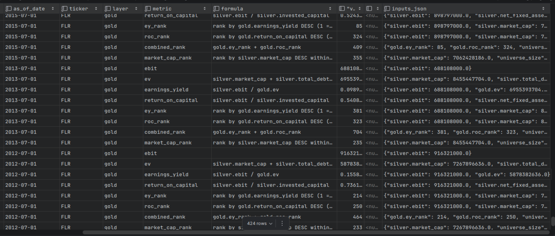
Every value is traceable. For example: earnings_yield for FLR on 2012-07-01, built from ebit / ev, where silver.ebit=916321000.0 and gold.ev=5878382636.0.
7. Automatic Parameter Optimisation: Optuna

Optuna is an open-source Python hyperparameter optimization framework. I used it to find the best values for the Sortino threshold and Piotroski minimum score. It’s much faster than brute force because it uses Bayesian search (TPE sampler) rather than testing every combination.
To guard against overfitting, I ran the strategy with the tuned parameters on different rebalance dates. First manually, checking each result. Then automatically across all 12 months (1st day of each month), generating a probability distribution.
_adv = advantage. Positive means the Magic Formula portfolio beat the IWB benchmark.
  [ 1/12]  Jan-01 ...  cagr_adv=-2.1%  mwr_adv=-4.3%  win_rate=38%
  [ 2/12]  Feb-01 ...  cagr_adv=-0.8%  mwr_adv=-1.6%  win_rate=25%
  [ 3/12]  Mar-01 ...  cagr_adv=-2.5%  mwr_adv=-3.6%  win_rate=38%
  [ 4/12]  Apr-01 ...  cagr_adv=+1.2%  mwr_adv=+0.8%  win_rate=50%
  [ 5/12]  May-01 ...  cagr_adv=-1.3%  mwr_adv=-1.7%  win_rate=44%
  [ 6/12]  Jun-01 ...  cagr_adv=+1.0%  mwr_adv=+1.2%  win_rate=50%
  [ 7/12]  Jul-01 ...  cagr_adv=+1.5%  mwr_adv=+1.9%  win_rate=50%
  [ 8/12]  Aug-01 ...  cagr_adv=+0.7%  mwr_adv=+0.6%  win_rate=44%
  [ 9/12]  Sep-01 ...  cagr_adv=-1.4%  mwr_adv=-2.6%  win_rate=56%
  [10/12]  Oct-01 ...  cagr_adv=-4.7%  mwr_adv=-5.1%  win_rate=38%
  [11/12]  Nov-01 ...  cagr_adv=-4.9%  mwr_adv=-5.8%  win_rate=31%
  [12/12]  Dec-01 ...  cagr_adv=-2.3%  mwr_adv=-4.0%  win_rate=44%
This particular run still had momentum enabled. The sweep revealed it was the culprit: momentum parameters that looked great on July rebalance collapsed on most other dates. That sensitivity to entry timing is the classic overfitting signal.
Once momentum was disabled and only Sortino and Piotroski were kept, the results stabilised. April, June, July, and August show the strongest months — consistent with known seasonal effects around earnings season. The final configuration used in Appendix 2 and 3 is July rebalance, which sits in that better-performing window.
8. Summary
- Beating the benchmark is hard.
- Beating it on historical data says nothing about the future. But it does show whether the method ever had an edge.
- Backtesting is hard. It involves a lot of assumptions and a lot of data. But once built properly, the framework can be reused for other strategies.
- Know what kind of investor you are. If my method slightly underperforms the benchmark but is more volatile, I might still prefer it. Consistently betting on value stocks in a volatile market is the kind of bet I want for my riskier portfolio.
- Benchmarks are powerful. Given that, it makes sense to hold multiple portfolios: one that simply tracks the benchmark, avoids all the risks mentioned here, and bets on a long horizon with no behavioral interference. And a separate portfolio for systematic stock picking, which works for me. It satisfies my need to do the math. It also solves the behavioral problem by delegating decisions to an algorithm, which means I’m less likely to sabotage my other portfolios where I use different strategies.
- Auditability is non-negotiable. A final ranking means nothing if you can’t trace how each number was calculated and spot-check a sample.
- Vanilla Magic Formula did not outperform Russell 1000 over the 16-year backtest. The method has been widely published; the edge is gone. With Sortino and Piotroski filters, the edge comes back: +4.8% CAGR over IWM (same universe) and +1.5% over IWB (large caps).
- The clearest lesson: regular investing works. Whether you use Magic Formula or just buy the benchmark, contributing \$320,000 over 16 years turned into over \$1M — vs \$794k for IWM and \$1.17M for IWB.
Appendix 1. Magic Formula Backtesting config
| start_year | 2010 |
| end_year | 2025 |
| rebalance_month | 7 |
| rebalance_day | 1 |
| top_n | 20 |
| benchmark_ticker | IWM |
| — Universe — | |
| universe_n | 2000 |
| universe_offset | 0 |
| — Filters — | |
| min_market_cap | 50000000 |
| max_market_cap | 0 |
| excluded_sectors | Financials, Utilities, Real Estate, Financial Services |
| excluded_industries | Insurance, Managed Care, Healthcare Plans, Insurance—Life, Insurance—Property & Casualty, Insurance—Specialty, Insurance—Diversified, Insurance Brokers |
| — Contributions & Fees — | |
| annual_contribution | 20000 |
| transaction_fee_pct | 0.001 |
| risk_free_rate | 0.04 |
| — Overlays — | |
| screens.sortino_min | 0.2 |
| screens.sortino_window_days | 252 |
| screens.momentum_sma_days | 0 |
| screens.momentum_lookback_months | 0 |
| screens.piotroski_min | 3 |
| screens.composite_value_top_pct | 0 |
Appendix 2. Magic Formula backtesting 2010 - 2025
IWB = Russell 1000 (large caps). IWM = Russell 2000 (small caps, same universe as portfolio).
| year | as_of_date | n_holdings | n_survivors | portfolio_return | IWB return | IWM return | annual_contribution | total_contributed | portfolio_value | IWB value | IWM value | portfolio_profit | IWB profit | IWM profit |
|---|---|---|---|---|---|---|---|---|---|---|---|---|---|---|
| 2010 | 2010-07-01 | 20 | 804 | 44.8% | 34.0% | 40.3% | 20,000 | 20,000 | 28,933 | 26,800 | 28,064 | 8,933 | 6,800 | 8,064 |
| 2011 | 2011-07-01 | 20 | 925 | -6.7% | 3.0% | -2.4% | 20,000 | 40,000 | 45,551 | 48,202 | 46,911 | 5,551 | 8,202 | 6,911 |
| 2012 | 2012-07-01 | 20 | 472 | 26.5% | 21.6% | 24.4% | 20,000 | 60,000 | 82,780 | 82,943 | 83,224 | 22,780 | 22,943 | 23,224 |
| 2013 | 2013-07-01 | 20 | 776 | 23.8% | 24.7% | 22.9% | 20,000 | 80,000 | 127,029 | 128,340 | 126,882 | 47,029 | 48,340 | 46,882 |
| 2014 | 2014-07-01 | 20 | 790 | 12.9% | 7.7% | 6.2% | 20,000 | 100,000 | 165,666 | 159,825 | 155,923 | 65,666 | 59,825 | 55,923 |
| 2015 | 2015-07-01 | 20 | 536 | -1.6% | 2.3% | -6.5% | 20,000 | 120,000 | 182,380 | 183,937 | 164,474 | 62,380 | 63,937 | 44,474 |
| 2016 | 2016-07-01 | 20 | 449 | 19.3% | 18.0% | 25.0% | 20,000 | 140,000 | 241,050 | 240,546 | 230,665 | 101,050 | 100,546 | 90,665 |
| 2017 | 2017-07-01 | 20 | 681 | 8.5% | 14.4% | 17.6% | 20,000 | 160,000 | 282,556 | 298,073 | 294,664 | 122,556 | 138,073 | 134,664 |
| 2018 | 2018-07-01 | 20 | 629 | 6.6% | 10.4% | -3.8% | 20,000 | 180,000 | 321,818 | 351,227 | 302,637 | 141,818 | 171,227 | 122,637 |
| 2019 | 2019-07-01 | 20 | 465 | -7.5% | 7.1% | -7.8% | 20,000 | 200,000 | 315,461 | 397,688 | 297,347 | 115,461 | 197,688 | 97,347 |
| 2020 | 2020-07-01 | 20 | 360 | 55.6% | 42.7% | 64.9% | 20,000 | 220,000 | 521,027 | 596,022 | 523,182 | 301,027 | 376,022 | 303,182 |
| 2021 | 2021-07-01 | 20 | 700 | -13.8% | -12.6% | -25.1% | 20,000 | 240,000 | 465,234 | 538,518 | 406,727 | 225,234 | 298,518 | 166,727 |
| 2022 | 2022-07-01 | 20 | 286 | 37.0% | 18.0% | 11.3% | 20,000 | 260,000 | 663,441 | 658,876 | 474,789 | 403,441 | 398,876 | 214,789 |
| 2023 | 2023-07-01 | 20 | 713 | 23.4% | 23.9% | 8.7% | 20,000 | 280,000 | 841,503 | 841,016 | 537,852 | 561,503 | 561,016 | 257,852 |
| 2024 | 2024-07-01 | 20 | 518 | 21.9% | 15.2% | 9.6% | 20,000 | 300,000 | 1,048,224 | 991,602 | 611,433 | 748,224 | 691,602 | 311,433 |
| 2025 | 2025-07-01 | 20 | 524 | 31.4% | 15.2% | 25.8% | 20,000 | 320,000 | 1,401,079 | 1,165,683 | 794,343 | 1,081,079 | 845,683 | 474,343 |
| Average | 601.75 | 17.6% | 15.3% | 13.2% |
Appendix 3. Magic Formula backtesting metrics
| Portfolio | vs IWB (Russell 1000) | vs IWM (Russell 2000) | |
|---|---|---|---|
| Annual Contribution | 20,000 | ||
| Transaction Fee (per leg) | 0.1% | ||
| Risk-Free Rate (annual) | 4.0% | ||
| Total Years | 16 | ||
| Total Contributed | 320,000 | ||
| CAGR (time-weighted) | 16.1% | 14.6% | 11.3% |
| CAGR Advantage | +1.5% | +4.8% | |
| MWR / IRR (money-weighted) | 15.9% | 14.0% | 10.0% |
| MWR Advantage | +1.9% | +5.9% | |
| Sharpe (annual) | 0.697 | 0.868 | 0.429 |
| Sharpe Advantage | -0.171 | +0.268 | |
| Max Drawdown | -13.8% | -12.6% | -25.1% |
| Win Rate | — | 50% (8/16) | 75% (12/16) |
| Final Value | 1,401,079 | 1,165,683 | 794,343 |
| Profit | 1,081,079 | 845,683 | 474,343 |
| Avg Survivors / Year | 601.75 | ||
| Min Survivors / Year | 286 |
- Positive CAGR and MWR advantage against both benchmarks. Against IWM (same universe): +4.8% CAGR, 75% win rate. Against IWB (large caps): +1.5% CAGR, 50% win rate.
- Sharpe is better than IWM (+0.268) but worse than IWB (-0.171). The portfolio takes on more volatility than large caps but less than small caps.
- Max Drawdown: much better than IWM (-13.8% vs -25.1%). The filters removed most of the worst small-cap crashes.
- Win rate 75% vs IWM. The strategy consistently picks better small caps than the index.
- Portfolio profit: \$1,081,079 vs \$845,683 (IWB) and \$474,343 (IWM). That’s \$235,396 more than large caps and \$606,736 more than the small-cap index over 16 years.
References
Sources:
- Magic formula investing - Wikipedia
- The Little Book That Still Beats the Market by Joel Greenblatt
- My personal backtesting and ETL pipeline framework (contact me at [email protected] if you’re interested in working together)